Graphs

 

There is a special object type in the T-FLEX CAD system - the "Graph". A graph is a function based on a set of points in its own two-dimensional coordinate system, connected by a polyline or by a smooth curve. This versatile instrument serves to define dependencies of different nature, for example, to specify a variable load in Analysis modules, or to create a parametric dependency based on an array of numbers from a database. Graphs are also used to store and display results of a dynamic motion analysis. Graphs can be used in the variables editor to read the values that they define. It is also possible to graphically define the laws of scaling or twisting in the "Sweep" operation, properties of an offset 3D path to define the offset distance, the variable radius value in the "Blend" operation.

Graphs are created and stored in the document together with the drawing and the 3D model. The system provides a specialized editor to create and edit graphs. It serves to manage arrays of points and their coordinates, supports multiple point selection as well as clipboard handling (copy/paste), undo/redo actions, axial zoom control, points dragging etc.

 

Creating and Editing Graphs

Graphs Manager

Working with graphs is done via a special dialog window - the "Graphs" manager, which displays the list of all graphs in the current document, and the buttons to start all required commands. The list of graphs is accessed via the command:

 

After calling the command, the "Graphs" window appears

To create a new graph, use the button [Create Graph…]. When creating a new graph, you are prompted to select the connection type of the graph nodes: by a spline (a smooth curve) or by a polyline. A newly created graph is empty. It is assigned its own name – "Graph_1", "Graph_2" etc. If desired, the user can modify the graph name using the button [Rename] or in its properties (see below).

The buttons [Delete] and [Delete All] serve to delete existing graphs from the current document.

 

Graph Properties

A dialog with descriptive and defining graph properties can be accessed by clicking the [Properties…] button in the graphs manager window.

The graph name and type are displayed in the upper part. You can edit the graph name. The graph type is defined at creation and is not changed later.

You can define the following graph properties in the "Units " parameters group:

●The labels for the graph's coordinate axes – in the fields "Argument Axis Title" and "Function Axis Title";

●The "Function/Argument Scale Factor" parameter defines the units scale along one axis relative to another one when plotting the graph. It is used to setup the image when individual axis scales need to be used. The graph editor can set this value automatically (see below);

     

●The "Minimal Argument Step" parameter determines the minimum allowed distance between two neighboring nodes of the graph in the X-direction.

The "Current Limits" group of parameters displays the information regarding the current graph bounds. You can also deliberately impose graph limits by the argument and by the function. When limits are enabled, the system will not allow creating points out of the limit bounds. By default, limits are not imposed.

The "Boundary Conditions" group of parameters defines the conditions for the ends of the graph line. Such parameters can be used only for the "smooth curve" graph type. You can define the tangent of the curve direction slope at the graph start and end. You can also set equalities of first and second derivatives at the graph start and end. Such boundary condition allows obtaining a smooth transition between copies when having a master graph segment repeated cyclically.

The "Read Only Mode" flag prohibits modifying properties and coordinates of graph points.

The "Show Nodes" flag enables the display of function nodes on the graph.

The "Show Limits" flag turns on graphic rendering of the range-of-definition bounds and the values range (actual) for the given graph. Graph bounds are displayed as a dotted frame.

The "Return Closest Fuctions Value for Arguments out of Graph Limits" flag serves to use the graph for any argument values, including those outside the existing defining range. This parameter is used to work with the function graph("GRAPH NAME", ARGUMENT VALUE) of the variables editor.

The flag “Logarithmic Argument Scale” sets the logarithmic scale along the argument axis of the graph.

The "Auto Repeat" group of parameters defines a cyclic repeating of a master graph segment in both directions. When repeating in the positive direction, then each copy of the master segment is attached by its start point at the end point of the graph, and vice versa when in the negative direction.

 

Graph Editor

Graphs are edited in a special graph editor. The editor is called by selecting the desired graph in the "Graphs" window and clicking the [Edit…] button, or by double-clicking on the graph's row. To simultaneously edit several graphs, select them into graphs manager using <Shift> and use the [Edit…] button as well. All graphs will be simultaneously displayed in the editor. At the same time, one of them will be active and editable. To switch between graphs, use the interface control (the drop-down list) with graph names.

The main portion of the editor window is occupied by the workspace, in which graphs are displayed. The workspace is ruled for convenience with an automatically scalable coordinate grid. Image moving (panning) and scaling (zooming) is done by the mouse wheel – in the same way as when drawing in T-FLEX CAD.

The coordinate rulers are displayed along the borders of the workspace. You can use these rulers in the same way as in the T-FLEX CAD drawing window – to pan and zoom the image. The graph editor allows separate zooming along the coordinate axes. Separate zooming is done using a ruler, when the appropriate mode is enabled in the graph properties, or by the icon on the editor's "View" toolbar. A specified ratio of coordinate axes units is automatically stored in the graph properties.

Clicking in the workspace creates a new graph point. All points are connected by a line (curve) of the specified type (a polyline or a spline). For user convenience, the current cursor position coordinates are displayed in the status bar in the lower-right corner of the graph editor.

At the right of the workspace there is the table of graph point coordinates. Point coordinates can be edited directly in this table. You can start editing coordinates after double-clicking in the desired table cell. To input changes, press <Enter> or switch the input focus to another window. The edited (selected) graph point is highlighted. To select several points, use the keys <Shift> or <Ctrl>.

A graph point position can be modified with the cursor, by "grabbing" the point with and dragging it to the new position. When double-clicking on a graph point, a special dialog appears to edit point coordinates. Here you can enter the absolute point coordinates (when switched to "position") or set offset coordinates with respect to the current point position (when switched to "offset"). If, when double-clicking , several points were preselected (for example, in the table of coordinates), then only the offsets can be used. This is convenient, if you need to "move" a segment of the graph by a certain distance (see an example below).

   

 

Graph Editing Tools

The graph editor has three bars with various tools and icons to launch utility commands.

 

The "Standard" toolbar contains:

●Commands to close the graph editor with or without saving changes:

       -        Save changes and close        

       -        Cancel changes and close        

●A drop-down list to select the name of the graph being edited is used when several graphs are edited simultaneously.        

       

●The command to save the edited graph in the external file:

       <Ctrl><S>        Save to File

●The “Download from file” command that allows us to replace the graph being edited with another graph from the external file “*.tflaw”. As a result of execution of this command all source points are removed, and the basic properties are replaced with other properties:

       <Ctrl><L>        Download from file

 

The "Edit" toolbar contains:

●An icon to call the edited graph properties dialog:

       <Ctrl><P>        Graph Properties        

●A drop-down list (combo box) to define the colors of the graph line:

       -        Graph Color        

●Commands to work with the clipboard:

       <Ctrl><A>        Select all nodes

       <Ctrl><C>        Copy        

       <Ctrl><X>        Cut        

       <Ctrl><V>        Paste        

To copy graph points to the clipboard, you first need to select points in the table of coordinates or in the workspace. Next, you can use the command "Copy" or "Cut". When copying graph points, the system must remember the reference point for future snapping when pasting from the clipboard.

To define the point, the "Copy…" dialog window appears. The user can define the coordinates of the reference point or select it on the graph. To select a point in the workspace, you need to enable the option "Show on Graph" and click [OK]. Next, the system goes into the mode of waiting for point selection. The respective help message appears at the bottom of the graph editor in the status bar line. The user can point at any location in the workspace or select any of the existing graph points. If the user did not specify a reference point, the system will use the origin instead.        

       

When adding the copied points from the clipboard to the graph, the system will prompt for defining the target point to snap the insertion to. The "Insert Nodes" dialog window will appear. In it you can also define the coordinates of the insertion target point or enable the mode of selecting such point in the workspace. If the user did not define the reference point at the time of copying, then, when defining the coordinates for the insertion, the user will thus define the offsets of the new graph points from the original position. When specifying the target point, the preview image of new graph points rubberbands with the cursor.        

       

●Commands to work with graph nodes:

       <Ctrl><N>        Add new Node by Coordinates        

       <Ctrl><E>        Edit Node Coordinates        

       <Del>        Delete Selected Nodes        

       <Ctrl><Shift><Del>        Delete All Nodes        

●Commands to undo unwanted actions and redo undone actions:

       <Alt><BackSpace>        Undo        

       <Ctrl><BackSpace>        Redo        

●Options to enable the modes of selecting nodes and object snapping:

       -        Mark / Select nodes        

       -        Snap to Nearest Point        

       -        Snap to Nearest Node        

       <Ctrl>        Move Nodes by Coordinate Axes        

 

The "View" toolbar contains:

●The command to refresh the image:

       <F7>        Update Window        

●Commands to zoom in and out the image:

       <Ctrl><Shift><PgUp>        Zoom In        

       <Ctrl><Shift><PgDown>        Zoom Out        

●The command to automatically fit the entire image within the workspace window bounds:

       <Ctrl><Shift><End>        Zoom All        

●Commands to pan (move) the image:

       <Ctrl><Shift><Left>        Left        

       <Ctrl><Shift><Right>        Right        

       <Ctrl><Shift><Down>        Down        

       <Ctrl><Shift><Up>        Up        

●The button to enable the mode of separate zooming by axes:

       -        Zoom separately by axes        

●The command to enable/disable the mode when a special vertical marker is displayed that reads the argument position and returns the respective function value. This command is duplicated with a special switch flag in the graph editor options (see below):

       -        Argument Marker        

●An icon to call the graph editor options dialog (see options description below):

       <Ctrl><O>        Options        

 

Setting Up the Graph Editor

The dialog contains interface controls to set up the graph editor appearance.

The "Show" group of options contains the switches to enable/disable auxiliary utility objects – the ruler, the automatically scalable coordinate grid, coordinate axes, the argument marker.

The pane in the "Current View" group of options displays the coordinates of the displayed area for the user reference.

The flag “Independent Zoom by Axes” controls the mode of independent scaling along the axes. If it is turned on, then upon scaling with the help of the ruler the visual scale factor along the X-axis changes independently of the scale along the Y-axis.

The flag “Logarithmic Scale by Argument Axes” is a reference flag and is always unavailable for editing. This flag shows what argument scale is set in the properties of the graph being edited.

In the right part of the dialog there is a group of controls to set up the colors of various objects in the graph editor.

With the help of the parameter “Ruler font size” you can also define the font size for the graph editor ruler.

 

Using graphs

As was mentioned in the beginning of the chapter, graphs can be used in various areas of the system. In this topic we will review specific examples of using graphs.

 

Using graphs in 3D operations

Graphs can be used for a more intuitive way of defining tabular dependencies in some 3D modeling commands. For example, in the "Blend Edge" command – to define the law of changing a variable radius, or in the "Sweep" operation – to define the law of changing the twist angle or scaling of the contour. It can be used wherever you need to define the law of changing some operation's parameter over a certain range, whose length is defined in percent (0%-100%).

To define a dependency by a graph, use the special "Graph" button in the operation properties window, next to the field for defining the entries of tabular dependencies. Upon clicking the button, the graph editor opens, in which there is already a graph constructed based on the input data. (By default, those are the point positions 0% and 100% with the respective parameters.) The graph type in this case is always a smooth curve.        

       

Depending on the operation type, we can distribute various properties using a graph. The definition range and the graph values range are also limited depending on the operation type. The range of values allowed for input in the X-axis is always from 0 to 100. This defies the position of each point. In the Y-axis we reckon the operation parameter values for each point. For example, for a variable round blend, one can define the law of the radius distribution along the span of the selected edges. In this case, the system will not allow setting the function value less than zero, since this is restricted in the blend operation.

       

To save the results of editing a graph, exit the editor by clicking the button . After closing the editor, the system will transfer all graph points to the properties window to display the dependencies in the tabular form.

 

Using Graphs in the Motion Analysis, in the Variables Editor

Graphs are used on several occasions in the «Dynamic motion” module:

1. To display the results of a dynamic calculation – to record the changing in time coordinates, forces, moments etc.

2. To define variables for loads, springs.

A prepared graph can be used in the variables editor for further calculations, by reading its function value in the variables editor using the expression graph("graph name", argument value).

Note that this chapter brings only the examples of using a graph in the dynamic motion calculations. For detailed information on the dynamic motion analysis refer to the respective chapter of the documentation.

As an example of a varying load, which can be defined using a graph, consider a motor (the "Torque" load), which turns on and off at a certain time instant. The graph for such load may look as follows:

Sometimes, one may need to define nonlinear properties in spring, for example, to account for an imperfect spring. At the extreme compression, when its coils contact each other, the rigidity increases manifold. One can also account for the spring destruction instant at a certain deformation level value (the spring elongation). At that instant, the spring resistance disappears. We shall clarify here, that the "destruction" of such spring in the model will be reversible, that is, when the model returns to a state with the spring elongation within the normal range, then the spring will automatically restore. The graph for such spring will define the dependency of the bipolar force on elongation and may look as follows:

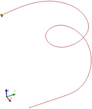
Let's review the use of graphs to record results of a motion analysis and using the function graph("GRAPH NAME", ARGUMENT VALUE) on an example of solving a typical problem of finding and maintaining an equilibrium of a moving body. For the example, we will create a simplified model of the "Waterslide" attraction.

 

Problem conditions. There is a spatial descending and trajectory (a 3D path). A body shall move strictly along this path under the gravity force. The problem is formulated as to design such a surface, along which the body could slide and follow the prescribed path. To simplify the example, we will use a ball as the moving body and neglect the friction force. Let's also skip some details of the design in the example description, which are not related to working with graphs.

The file with this example is located in library “Examples/3D Modeling/Graph/Waterslide.grb”.

       

To solve this problem, you need to have the dynamic motion module installed.

 

The solution to this problem is obtained in several steps:

1. The ball shall be made moving under the gravity force along the specified path (as if on a rail). At the same time, it is necessary to remember the extra G-forces acting on the ball. We will create the first motion analysis study for this purpose. We can collect all necessary data in the way of graphs.

2. Adjusting the results of the motion analysis, creating variables, reading graphs.

3. Constructing the ball path.

4. Constructing the surface.

5. Verifying the result. Creating the second motion analysis study.

Step 1. To create a dynamic motion study, we will need to create one "Coincident" mate, which will bind the ball (the center of gravity) to the trajectory (the 3D path). To read the results, we will need two sensors. To record the changing in time reaction force (the extra G's) we will need a joint sensor (joins are created automatically based on mates). To record the coordinates of the ball position, we will need a "point" sensor (at the ball's center of gravity). As the result of the motion analysis, we will record in the way of graphs the following values:

· the graph "Х, Point of Rotation_0 Body" - records the X-coordinate of the ball position Х;

· the graph "Y, Point of Rotation_0 Body" - records the Y-coordinate of the ball position;

· the graph "Z, Point of Rotation_0 Body" - records the Z-coordinate of the ball position;

· the graph "RF_Joint_0" - records the magnitude (vector length) of the reaction force in the joint_0;

· the graph "RFX_Joint_0" - records the X-component of the reaction force in the joint_0;

· the graph "RFY_Joint_0" - records the Y-component of the reaction force in the joint_0;

· the graph "RFZ_Joint_0" - records the Z-component of the reaction force in the joint_0.

Step 2. Create several variables to read the values from graphs in the variables editor. The function graph() will be used in the expressions. The {a} variable will be used as the time counter. All events of interest occur in the time period from 0.008 to 1.4 seconds with the step of 1/125. The variables are recorded as shown on the following figure. The function graph()can read values from graphs using the time counter {a}.

Step 3. By using the variables {XX}, {YY}, {ZZ} we can re-create the ball's center of gravity position at any time instant by varying the {a} variable.

The tools that we use (a 3D path with the parametrically changing 3D node, a parametric sweep), can only use an integer counter and vary it with the step equal to 1. Therefore, the variable {a} will be varied with the help of another counter {t}.

The variables {fx}, {fy}, {fz} will be assigned the coordinates of the reaction force unit vector, therefore those can be used to define the direction of the extra G-force action. Let's create a 3D node and enter these variables instead of the coordinates. Additionally, we need to account for the ball radius, therefore we introduce a correction to the coordinates as 5*(fx,fy,fz). This node will be changing its position along with the varying variable {t} Next, based on the new 3D node, construct a parametric 3D path by varying the counter {t} in the range from 1 to 175 (at the same time, the time counter {a} will sequentially read all values from graphs). This new path (3D path_1) renders the line of contact between the ball and the surface which we need to construct. It will also be needed to correctly position the "movable" profile for the prospective surface.

       

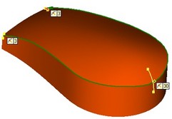
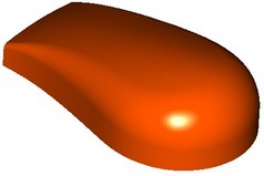
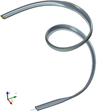
Step 4. To construct the surface using the "By Parameters" operation, we need a "movable" profile. We can bind it to our "movable" 3D node by creating in it a local coordinate system (LCS). To define the direction of one of the LCS axes, we will create an offset 3D node in the force vector direction (by defining the coordinates (fx,fy,fz) relative to the source 3D node). The second LCS axis will be set tangent to the 3D path_2. By having a "movable" profile, we can create a parametric sweep by varying the {t}-counter operation parameter in the range from 1 to 175.

Step 5. Result verification. Create a new motion analysis study and release the ball on the created surface; it will exactly follow the claimed path, meaning that the created surface fully satisfies the problem requirements.