Optimization


Optimization |
|
T-FLEX CAD provides a capability for computing parameters of a 2D drawing or a 3D model by solving an optimization problem under certain constraints on the model variables. The solution to this problem yields a set of values for the existing variables that satisfy the imposed conditions best.
Main concepts
Optimization of the model is done by using the command "PO: Optimize Model":
Icon |
Ribbon |
|---|---|
|
Parameters → Tools → Optimize |
Keyboard |
Textual Menu |
<PO> |
Parameters > Optimize |
The command is accessible only when numerical variables are present in the document.
Calling the command brings up the dialog box "Optimization Task", that contains the list of the defined optimization problems. The column "Name" displays the name of the variable, whose value is optimized by the current task. The column "Comment" contains textual strings entered by the user.
A T-FLEX CAD document may contain any number of optimization tasks.
The graphical buttons at the bottom of the dialog box allow the following actions:
Add. Entering a new optimization task.
Delete. Deleting the task of the current list item.
Properties. Displays "Optimization Parameters" dialog box of the current list item task.
Run. Starts the optimization computations. The system seeks for the solution according to the specified optimization parameters and regenerates the drawing or the 3D model with the found variable values.
Close. Exits the command.
Optimization task definition
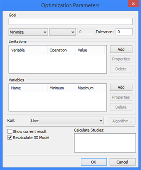
Upon pressing the [Add] button, the "Optimization Parameters" dialog box is displayed that contains the following fields:
Goal. Keeps the textual string that is the comment of this optimization task. Next are the combo box for selecting the target function (Make Equal, Minimize, Maximize), the variable Name combo box and the Tolerance input box. The variable is selected from the list containing all numerical variables present in the document. If the selected function type is "Make Equal", then the input box becomes accessible for entering the target value of the variable.
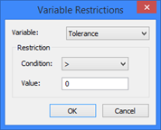
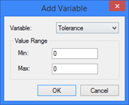
The tolerance value defines the admissible range of the values of the target variable within which the optimization task is considered solved. Limitations. Defines the list of restrictions on the model variables when performing the optimization. New limitations are entered upon pressing the [Add] button. In the "Variable" box, set the name of the desired variable (one variable can be subject to multiple restrictions). In the "Condition" combo box, select one of the comparison types (<, >, <=, >=) for comparing the variable against the target value (the "Value" input box). To modify the entered limitations, use the button [Properties] that allows editing all fields of the current line in the limitations list. Pressing the [Delete] button deletes the current line of the limitations list. Variables. This is the list of variables whose values will be the subject to the optimization process. The range of admissible values is to be defined for each variable. To be formulated correctly, the optimization task requires defining the range of admissible values for at least one variable. The graphic buttons [Add], [Properties] and [Delete] work similar to those described in the previous section. To define a new record, you need to fill in the following entries: Set the variable name by selecting from the list in the "Variable" combo box (each variable can have only one the range of admissible values). |
|
The entries "Minimum" and "Maximum" define the bounding values of the variable's range of admissible values. When solving the optimization task, the values of the variables are tried that satisfy the set of the limitations and fall in the range of admissible values. Once a limitation is defined for a variable, its name is no longer available for defining the range of values, and vice versa. The variable whose value is the target of the optimization is not included in the lists of variables when defining limitations and the value ranges. |
|
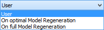
Run. This parameter takes one of the following values: User. The optimization task will run only upon user pressing the bottom [Run] in the "Optimization Task" dialog box. |
|
Optimizing may take long time on complicated drawings or 3D models. The described setting allows skipping optimization when regenerating the model.
On optimal Model Regeneration. The optimization task will run upon partial (optimal) model regeneration (when only modified elements are regenerated).
On full Model Regeneration. The optimization task will run upon full model regeneration.
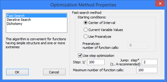
To select an optimization algorithm and to define its parameters, use the graphic button [Algorithm…]. Pressing this button brings up the dialog box for defining the algorithm parameters.
The pane in the left side of the dialog box displays the list of available optimization methods: Fast Search. This method is suitable for functions with one or two extremes. Dichotomy. This method is suitable for functions of one variable. Not recommended for handling restrictions Iterative Search. This method is suitable for functions with complicated behavior and multiple extremes. The right side of the dialog box contains the set of parameters for the selected optimization method. The button [Ok] closes the dialog box, saving the entered changes. The button [Cancel] allows quitting the dialog box without saving changes. |
|
Show current result. If this flag is set, the "Finding Solution" window dynamically displays the variable values as the solution progresses.
Recalculate 3D model. Setting this flag forces the 3D model regeneration at each step of the optimization algorithm. If the target function of the optimization (the variable) is related to 3D elements, then this flag is required for proper optimization process.
Examples of using optimization
Idler roller positioning task
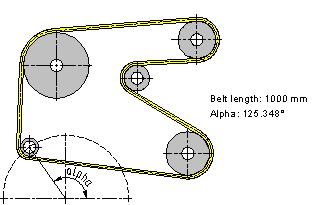
As an optimization example for a 2D model, let's consider the task of finding an idler roller position for fitting the belt of a specified length. This example can be found in the library "Examples \2D Design\Optimization\ Belt.GRB".
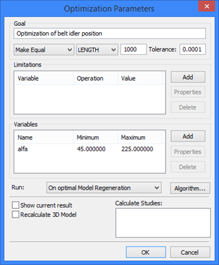
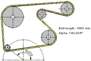
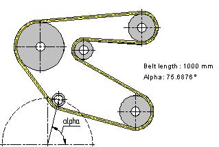
The example presents a kinematic system of a generic belt drive. Let's assume one of the requirements for the design of the system being the fixed belt length (1000 mm), adjusted by the position of an idler. The idler position depends on the angle of turning its mounting bracket. The turning angle of the idler mounting bracket is defined on the drawing by the parameter of the respective construction line created as "through node, at an angle to horizontal". This parameter of turning the construction line was defined by a variable named "alpha". The length of the belt is defined by the variable "Length". Let's define the optimization task for this model by calling the command "PO: Optimize Model". The target condition will be the equality: the variable "Length" is equal to 1000 mm with the tolerance 0.0001. Let's set to the variable "alpha" to be the target of the optimization, with the values ranging from |
|
Upon defining all optimization parameters, any change in the drawing will trigger the optimization. For example, moving any of the rollers or changing any radius requires running the optimization to define the position of the idler. Meanwhile, the belt length is maintained equal or nearly equal to 1000 mm.
Bottle volume optimization task
This example clarifies use of optimization for 3D models. The file for the example is located in the library "Examples \2D Design\Optimization\ Bottle.GRB".
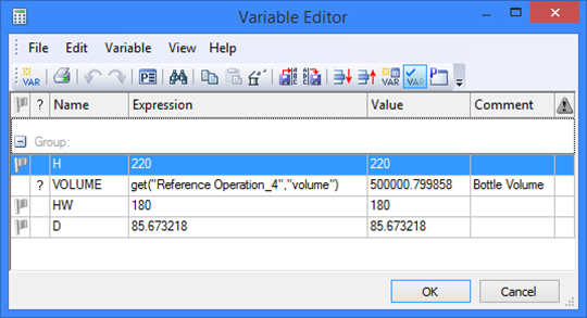
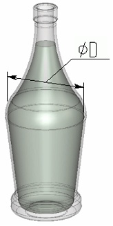
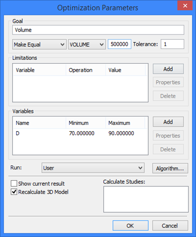
The example presents the solution to the bottle volume problem. In this example, the variable "Volume" is created, equal to the bottle capacity, that is, the volume of its contents. The variable "H" defines the height of the bottle, while "HW" – the level of the liquid in it. The optimization task is to maintain the constant bottle capacity (0.5 liter = 500000 mm3) while varying the bottle height and the level of the liquid in it. To achieve this goal, we need to find the value of the variable "D" driving the median diameter of the bottle (the widest portion diameter). The optimization task "Volume" was defined in the command "PO: Optimize Model" as follows. The target function equates the variable "Volume" to 500000 with the tolerance equal 1. The modifiable variable is "D", in the range from 70 to 90. No additional conditions are imposed on the model variables; therefore, no restrictions are defined. To visualize the optimization process, the flags are turned on, "Show current result" and "Recalculate 3D model". The dichotomy method is selected for the optimization algorithm, with the maximum number of iterations equal to 100. The parameter "Run" is set to the option "User", so that the optimization is run only upon the user request. |
|
After specifying the optimization task, let's modify the model. For example, let's reduce the bottle height and, respectively, the level of the liquid in it, by changing the values of the variables "H" and "HW". This reduces the capacity of the bottle.
To adjust the bottle diameter, simply call the command "PO: Optimize Model", select the task "Volume" in the coming up dialog box and press the graphic button [Run]. The shape of the model will be changing on the screen according to the current values of the variable being optimized as the solution progresses.
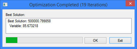
By accepting the found solution by pressing the button [Ok], we get the bottle 220 mm high and 0.5 liter in capacity.